Real-time inference for JEPA world model architectures with Ray

With V-JEPA2-AC the system decides what a robot arm should do next by assessing hundreds of possible futures and picking the one closest to the goal. It takes a significant amount of time between moves. This document presents a design and tested implementation for getting that under a second by moving the search into a Ray cluster.

Link01 · A Primer on Robotics

A robot perceives a partial observation of the environment, selects an action via some policy, executes it through a controller, and repeats this at control-loop frequency. Classically, each of those three functions is solved in closed form, and a CPU on the robot is enough to run all of them.

Classical robotics built each of those three boxes from first principles: hand-derived kinematics for perception, trajectory optimization for planning, PID or model-predictive controllers for control. This approach, depicted in Figure 1, underlies decades of industrial automation, but every new task, object, or environment typically requires new engineering.

Classical robotics — ~1 ms / action

Figure 1. The loop every robot runs. Perception turns sensor readings into state, planning produces a path, control executes it, and the arm closes the loop through the physical world. All three are solved in closed form on one on-board CPU. What it costs is engineering: the policy only covers the task it was derived for.

Physical AI aims to replace some or all of those boxes with networks trained on data, trading hand-derived precision for generality: a model trained on sufficient data transfers to situations not explicitly programmed for.

LinkHow the JEPA architecture fills the "plan" box

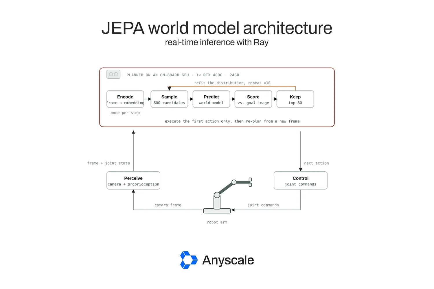
V-JEPA2-AC is one such model. It is built on the Joint-Embedding Predictive Architecture (JEPA). In this architecture, the system decides what a robot arm should do next by assessing hundreds of possible futures using the model and picking the one closest to the goal. Figure 2 shows the whole loop in place on the hardware that runs it.

Deployed zero-shot on Franka arms in two labs, with no fine-tuning for the specific environment, V-JEPA2-AC reports 65–80% success on pick-and-place with novel objects. This ran on a single RTX 4090. However, that configuration takes 16 seconds to plan every single action. It is not fast enough to run continuously.

LinkWhere the sixteen seconds actually goes

It is worth walking one planning step end to end, because the arithmetic explains the rest of this document. The arm holds still. The camera frame and the goal image are encoded once. The search algorithm, CEM, then draws 800 candidate action sequences from a Gaussian centered on its current best guess, pushes every one through the predictor, scores the results against the goal embedding, keeps the best 80, and re-centers the Gaussian on them. That is one round, and it happens ten times: roughly 8,000 predictor evaluations for one small movement of one arm. The system then executes only the first action of the winning sequence, throws the rest away, and starts over from a fresh frame. The cost is structural, and it recurs at every step.

V-JEPA2-AC on one on-board GPU — 16 s / action

Figure 2. Only the plan box changes. The robot still captures a camera frame and its joint state, and control is untouched, but the closed-form planner is replaced by the model and a search around it. The encoder is part of the model, so encoding happens here, once per step; the ten-round loop that follows is the expensive part.

The controller is also blocking: it waits for the previous action to complete before sending the next, so planning never overlaps with motion. The robot pauses, plans for sixteen seconds, moves, and pauses again. That stutter, not the model's accuracy, is the problem this document sets out to fix.

Link02 · The Approach

We take the approach of, first, moving world model inference off the robot and into a cloud server. While this introduces the new cost of a network round trip on every control step, that is offset by other improvements. First, it opens the opportunity of serving the model on a more powerful GPU. In this implementation we use NVIDIA A100-40GB GPUs, which have more memory than the 24 GB RTX 4090 used in the paper and substantially more bf16 throughput.

The same search on one cloud GPU — 21.4 s / action (measured, A100, optimized model)

Figure 3. The plan block lifts the inference off the robot. What stays local is sensing and actuation, so what crosses the network is one camera frame plus its joint state, and one action vector back.

On its own, a bigger GPU is not enough. Meta's reference planner, run unmodified on one A100 with these settings, takes 81.8 s per action; with the model-level optimizations in Section 05 it takes 21.4 s. Our 81.8 s is slower than the paper's 16 s on a 4090 because we ran Meta's released planning code as-is (fp32, 800 candidates × 10 rounds, a two-step horizon); the paper's timing likely reflects different settings or precision. Every speedup in this post is measured against our own 81.8 s baseline on the same hardware. Faster, but the arm still stops between moves.

The second step is to distribute the load across multiple GPUs. The opportunity comes from noting that within a single CEM refinement round rollouts can be computed independently and gathered before the round moves on. The paper runs them as one large batch on one GPU; nothing requires them to stay on one GPU. In our implementation we use one eight-GPU node (8× A100-40GB) on Anyscale.

The search distributed across a Ray cluster — 2.86 s / action (measured, 8× A100); 0.86 s with 3 rounds per step

Figure 4. One step inside the plan block changes. The 800 candidates in a round are independent, so the predict step fans out across warm replicas that already hold the model and gathers before scoring. The ten rounds are still sequential, which is what sets the floor.

We implement this using Ray.

Link03 · A Primer on Ray

LinkA general framework for turning Python into a cluster program

Ray is an open-source framework, originally built at UC Berkeley's RISELab and now maintained by Anyscale, for scaling ordinary Python from a laptop to a cluster without rewriting it as a distributed system. It exposes a small set of primitives and preserves mostly-sequential code structure.

LinkRay Core

Ray Core has two building blocks that matter here. A @ray.remote function becomes a task, scheduled somewhere in the cluster and returning a future. A @ray.remote class becomes an actor: a stateful worker pinned to a machine, and optionally a GPU, that keeps loaded model weights resident between calls. Tasks suit one-off parallel work; actors suit a process that pays to load a 1.2-billion-parameter checkpoint once and then answers many cheap requests.

LinkRay Serve

Ray Serve sits on top of Ray Core: a @serve.deployment declaration is enough for Ray to manage a pool of replicas, route requests, and scale under load. Ray Core answers how to run a function on many workers; Ray Serve answers how to expose it as a service other systems call, which is the shape a robot's control loop needs, a low-latency endpoint hit once per step.

Link04 · Implementation

LinkTwo Ray Serve deployments, composed

The design is two Ray Serve deployments and a handle between them. WorldModel is the GPU tier: one replica per GPU, each holding the encoder and predictor (we ran 8 replicas on 8 A100s). Planner is the driver: it runs the ten-round CEM loop, fans each round out across those replicas, and serves the endpoint the robot calls once per control step. Composing them this way, rather than as loose Ray Core actors, puts them under Serve's control: placement, health checks, restarts, and a declarative config a KubeRay RayService can roll out without downtime. The shape below elides the internals; what matters is where the fan-out sits. See figure 5 for a diagram of the deployment layout.

serve_app.py — Ray Serve · the shape, details elided

Two choices carry the design. The GPU tier is pinned at num_replicas=8 rather than autoscaled, because a search whose replica count changes mid-round has unpredictable latency, and the point is a stable per-step budget. max_ongoing_requests=1 makes each replica take one shard at a time, so an 8-way fan-out lands one shard per GPU instead of queueing several on a subset. Underneath, each replica is still a Ray Core actor, which is why the weights stay resident; the difference is that Serve owns the lifecycle.

Figure 5: Ray Serve on Anyscale connects the robot-facing Planner deployment to warm WorldModel replicas through a DeploymentHandle, with one model

What we learned building it. Three details decided the latency. First, the observation and goal latents (2.8 MB) go into Ray's object store once per plan with ray.put; every replica reads them from shared memory and caches them on its GPU, so each round moves only about 5 KB of candidate actions out and the energies back, and Ray's whole share of a round (fan-out, gather, refit) is under 10 ms. Second, with max_ongoing_requests=1 Serve's default power-of-two-choices router occasionally placed two shards on one replica while another sat idle, doubling that round; Serve's round-robin request router lands the shards of a round on consecutive replicas, one per GPU (zero collisions in 50 rounds). Third, our Serve replica processes started with TORCHDYNAMO_DISABLE=1 in their environment, which silently turned torch.compile into a no-op; clearing it in the replica's constructor recovered a 1.35× speedup.

Source. The full implementation, including model loading, the fast scoring path, the complete CEM refinement step, the two Serve deployments, every benchmark script and a runnable notebook, lives in the companion repository: https://github.com/anyscale/robotics_world_model_inference/tree/main/v3_realtime_inference_for_jepa

Link05 · Results

LinkMeasured on 8× A100

We built the design above and measured it on one Anyscale node with eight A100-40GB GPUs, using the search settings from Section 01 (800 candidates × 10 rounds, keep 80, horizon 2). The anchor is Meta's reference planner, run unmodified in fp32 on one A100: 81.8 s per action. Before adding GPUs we made the model itself faster on one GPU: a KV cache across rollout steps (the predictor is frame-causal, so earlier frames never need recomputing), bf16 with FlashAttention, and torch.compile. The result matches the reference energies (Pearson r = 0.9999) and brings one GPU to 21.4 s per action, 4× faster.

Figure 6. Measured planning time per action. Ray Serve fans each round out over 8 A100s (2.86 s, 29× the reference). Running 3 search rounds per step instead of 10 reached the same accuracy in closed-loop tests (Section 06), giving 0.86 s per action, 96× the reference.

Then the fan-out. Each round's 800 candidates are split across W WorldModel replicas, one GPU each. Going from 1 to 8 GPUs cuts a plan from 21.4 s to 2.86 s, a 7.5× speedup. Same seeds give identical plans at every GPU count, so sharding changes the speed of the search but not its answer. The latency model proposed in the first draft of this post holds up: calibrated on our measured single-GPU round (2.14 s), it predicts 2.94 s at 8 GPUs against 2.86 s measured.

LinkPlanning latency vs. cluster size

A100-40GB replicas on one 8-GPU node. Points are measured; the line is the latency model.

2.86 s / action at 8 A100 workers. This is 7.5× faster than one A100 and 29× faster than Meta's reference planner.

Figure 7. Plan latency vs. number of GPU replicas, measured on 8× A100 (points) against the latency model calibrated on the measured single-GPU round (line; dashed beyond 8 GPUs = projection).

Model: time(W) = 10 × ( r / effective(W) + 0.001s × (W − 1) ), where effective(W) = W / (1 + 0.008×(W−1)) and r is the measured single-GPU round, 2.14 s on an A100. Beyond 8 GPUs the curve flattens, because each GPU's share of the 800 candidates gets small. Larger clusters pay off mainly by serving more robots, or larger searches, from the same tier.

Two things remain unmeasured: network latency between an on-premises robot and a cloud region, and performance on a physical arm (our closed-loop tests use the world model as the simulator). Cold start stays off the request path: replicas load and compile in about 50 s at deploy time, before they take traffic. Batching candidates differently does not change accuracy: the plans are identical at 1, 2, 4 and 8 GPUs.

Link06 · Further Optimization

LinkWhat to try once the search itself is no longer the bottleneck

Once each round is as fast as the GPUs allow, what remains is the chain of ten sequential rounds, and the next gains come from restructuring the loop rather than adding GPUs.

LinkA. Non-blocking control

Start planning step t+1 while the robot is still executing step t. That hides planning latency behind execution time instead of adding to it, and it is a controller change, not a model change.

Measured. We simulated an arm that takes 1 s per action and lands with 4 mm of execution error. A blocking controller spent 1.86 s per step (plan, then move). Non-blocking control, planning step t+1 from the world model's prediction of where step t will land, spent 1.04 s per step, i.e. the motion itself plus 40 ms. It reached the same final accuracy, and a 12-step episode took 15.3 s instead of 25.3 s.

Figure 8. Closed-loop episodes toward a goal 21.6 cm away, with the world model standing in for the robot. Left: 3 search rounds per step reach the same accuracy as 10 in a third of the planning time. Right: non-blocking control removes the planner from the robot's critical path.

LinkB. Warm-started CEM

Receding-horizon control throws away everything but the first action. Re-using the rest to seed the next step's distribution, instead of a fresh Gaussian, lets each replan converge in fewer than ten rounds, shrinking the sequential chain parallelism cannot touch.

Measured. In closed-loop tests, 3 rounds per step (0.86 s on 8 A100s) reached the same accuracy as the full 10 (2.83 s): both settle about 4 cm from a goal that starts 21.6 cm away. Warm-starting from the previous plan worked, but on this task a fresh 3-round search did equally well, so the gain came from running fewer rounds. How many rounds a task needs is worth tuning per task.

LinkC. Fleet-level batching

A GPU tier sized for one robot is idle between its requests. Behind a Serve endpoint the same tier serves a fleet, and request batching can pack shards from different robots into one GPU batch, amortizing the same warm GPUs across many arms.

LinkD. Model compression

Distilling or quantizing the predictor shrinks the compute term itself, independent of how many workers it is split across. It stacks with distribution rather than competing with it.

LinkE. Serving-level optimization

The predictor rolls forward step by step over the horizon, so what LLM serving already relies on carries over: KV caching across rollout steps, prefill and decode disaggregation, continuous batching. These shrink the same compute term from a different direction, inside the same Serve deployment.

Implemented. KV caching across rollout steps, together with bf16, FlashAttention and torch.compile, is part of the measured system. It gives 4× on a single GPU and matches the reference energies to r = 0.9999.

Link07 · Takeaways

The sixteen seconds is not an implementation defect. It follows from a deliberate architectural choice: a JEPA model predicts state rather than actions, so an action has to be searched for at inference time instead of read off a policy head. That is the same trade agentic systems make when they sample many candidates and score them, and it comes with the same benefit, a system that can be pointed at a new goal without retraining.

The four setups make the trade concrete. A hand-written policy buys millisecond actions and pays for them in task-specific engineering. V-JEPA2-AC trades that speed for a system that accepts any goal you can photograph. Moving the search to a cluster buys the speed back without giving up the generality, and does it in infrastructure rather than in the model. Measured on one node of eight A100s, Ray Serve takes the full search from 82 s to 2.9 s per action, with distribution doing most of the work and Ray adding under 10 ms per round. The ten sequential rounds set the floor that more hardware cannot move. Attacking that floor with fewer rounds per step brings it to 0.86 s, and non-blocking control hides what remains behind the arm's own motion.

LinkReferences

• Assran, M. et al. V-JEPA 2: Self-Supervised Video Models Enable Understanding, Prediction and Planning. arXiv:2506.09985, 2025. arxiv.org/abs/2506.09985

Assran, M. et al. V-JEPA 2: Self-Supervised Video Models Enable Understanding, Prediction and Planning. arXiv:2506.09985, 2025.

• Meta AI. Introducing the V-JEPA 2 world model and new benchmarks for physical reasoning. ai.meta.com/blog/v-jepa-2-world-model-benchmarks

Meta AI. Introducing the V-JEPA 2 world model and new benchmarks for physical reasoning.

• Ray Project. Ray Core: Key Concepts, Tasks and Actors.

Ray Project. Ray Core: Key Concepts, Tasks and Actors.

• Ray Project. Ray Serve documentation. docs.ray.io/en/latest/serve

Ray Project. Ray Serve documentation.

• Ray Project. KubeRay: RayService. docs.ray.io/en/latest/cluster/kubernetes

Ray Project. KubeRay: RayService.

Planning-time and success-rate figures are as reported in the V-JEPA2-AC paper (arXiv:2506.09985). Cluster sizing, the CEM parallelization design, the latency model, and all code shown are an independent engineering implementation built on top of that published work, not affiliated with or endorsed by Meta AI or the Ray project. Latency measurements in Sections 05 and 06 were taken on one 8× A100-40GB node on Anyscale (November 2026); the extension of Figure 6 beyond 8 GPUs is a projection.