In brief
As part of our broader focus on agent optimization, we’ve released a study demonstrating the efficacy of both horizontal and vertical scaling strategies for SWE agents. However, in our experiments, we have traditionally applied a uniform compute budget across problems, as if every task shares the same difficulty.
But outside of a controlled lab setting, that assumption doesn’t hold up.
In reality, we know that task difficulty follows a heavy-tailed distribution: a meaningful fraction of tasks are solved on low effort, while others require a large budget. For example, in a previous post detailing our efforts reaching a state-of-the-art result on SWE-rebench, we found that roughly 50% of tasks sampled from that benchmark are resolved by a single rollout of GPT-5.2, yet our original policy was spending five rollouts on every single one of them. That’s money being left on the table.
At a moment when so many companies are examining their token consumption and looking for ways to eliminate cost, we present our latest research: budget-aware execution strategies that can be adapted according to task difficulty, so you only spend more when you need to. Continuing our work on SWE-rebench, we show how cascading and parallel execution strategies, both paired with early stopping, let you optimize for cost or speed, while keeping quality still; cascading saves you the cost of the last rollout, while parallel execution spares you the wait time for the last rollout, as visualized in the illustrative diagram below. In this post, we cover how we designed these execution strategies and the results we got back.
Overview: Our existing SWE multi-agent architecture
Before digging into those execution strategies, let’s first recap the agent architecture we’re working with (see diagram below). A full overview can be found in our previous piece on how choosing the right SWE agent execution strategy helped us reach state-of-the-art on SWE-rebench, yet here are the basics:
- Parallel generation: Per query, our agent generates N candidates patches (rollouts) in parallel, with the final step of each rollout including a self-confidence score. At the same time, a test agent writes and collects tests that a correct patch should satisfy.
- Filter: Any candidates that fail the collected tests are eliminated.
- Extract: Repository source code relevant to the remaining candidates is extracted.
- Reduce: Agent selects a single, final candidate from the filtered and context-enriched pool.
Since rollout generation is both the dominant cost and parallelizable, it is the primary lever we experiment with in this work by controlling the number of rollouts and the order in which they run.
Adapting best-of-N execution strategies for SWE agent tasks
Working on benchmarks such as BrowseComp-Plus and DeepResearch-Bench, we’ve already explored different execution strategies that utilize the agent’s self-confidence to decide how much compute we invest in each task, including:
- Cascading with early stopping (cost-optimized): Start with cheap models and only escalate to more expensive ones if they fail or express low confidence; the cost savings from cheaply handling easy queries offsets the cost of the expensive model on the challenging long tail.
- Parallel execution with early stopping (latency-optimized): Fire all rollouts at once; once an acceptable candidate is identified, any rollouts still in progress can be terminated immediately. This avoids paying for completions that will never be used, and on queries that are resolved confidently early.
In the above execution strategies, we assumed that each candidate solution can be evaluated in isolation. However, as we found in our last publication on SWE-rebench, selecting a candidate based on individual self-confidence scores alone is noticeably inferior to using an LLM Judge (otherwise known as a selector). Instead of analyzing a single candidate, the selector reviews the entire pool of generated candidates alongside the relevant source code before making a final choice.
Because the selector relies on this holistic view, we had to adjust our approach. We can no longer simply ask, “Is this individual solution good enough to stop early?” Instead, our acceptance criteria must shift to a group dynamic: “Do we have a good-enough pool of candidates for the selector to successfully work with?“
Predicting the selector’s performance
This shift changes how we validate our pipeline. Because the selector makes the final choice or synthesis from a collective pool, we need a way to confidently predict whether that pool contains enough signal for the selector to produce a good result (the only exception is if the list contains a single candidate, in which case a selector isn’t needed anyway).
We found that two predictions were needed to inform the overall prediction of selector aptitude:
- Prediction #1: That running a selector on the list of candidates will solve the task. We called this prediction Resolve-Now (RN), calculated by a dedicated classifier – with a calibrated threshold p_target (p for precision) – which we trained for this purpose.
- Prediction #2: That generating more candidates, and then running a selector, will solve the task. We called this prediction Resolve-Later (RL). We calculate it by training another classifier to predict the likelihood of a selector running on a larger batch of candidates to solve the task, and subtracting Resolve-Now from it, giving us an estimate for the marginal gain of generating another batch of rollouts. We learn a calibrated threshold g (g for gain) for it as well.
If either p_target or g pass our threshold, we take that as a signal that there’s a good enough list of candidates at that moment. If that’s the case, we stop generating more rollouts and proceed in our pipeline. Importantly, p_target and g are parameters we can play with based on our own criteria; for instance, raising p_target’s threshold or lowering g’s threshold makes early stops less frequent, but safer (more expensive, yet more accurate).
Generating more signal
However, we found that self-confidence is not a strong enough signal to decide when to stop an SWE task early. We would need to generate some more features for our classifiers to more confidently make an early-stopping call. Here are some of the features we engineered:
- Test agent: As mentioned earlier, this is the agent that runs at the same time as the parallel generation phase, writing and collecting tests a patch should satisfy and running them against each candidate. Powered by a smaller, cheaper model (GPT-5-Mini in this case), its output – how many tests passed or how many candidates passed all tests – is crisp, easy to aggregate, and cheaper than a single extra rollout.
- Patch consistency: The variation in the git patches generated by our rollouts.
- Repo search consistency: The variation and coverage of the paths in the repository searched in our rollouts.
- Other metadata: The number of steps taken by the agents, the tool-error rate, and other metadata.
We can then compile them to a feature vector and feed them to our classifiers in order to predict RN and RL. The strongest among this features list are the self-confidence and the test-based features; however, even these are still mediocre, since predicting whether a SWE patch is correct is genuinely difficult.
Fortunately, though, we don’t need a perfect classifier to make successful stop decisions – we just need a calibrated tail.
Results
Part I: Cascading with early stopping (cost-optimized)
To adapt the cascade strategy mentioned above to the SWE agent setting, we performed the following steps:
- Predefine a sequence of N values (for example, [1, 3, 5]).
- Run N=1 rollout and wait for it to finish
- Evaluate our RN and RL classifiers to decide whether to stop or generate more runs.
- If the classifiers are not confident enough to stop, we launch more rollouts to reach our next N value (N=3), evaluating our classifiers again to decide whether we should stop.
- This “cascades” until we stop or hit our fallback maximum N, 5 in this case.
Applying the cascade execution strategy to our SWE agent, with N values of [1, 3, 5, 10], we see that more than 50% of the tasks are stopped early, spending only a fraction of our full budget:
We evaluated our results on the same SWE-rebench dataset slice we used in our previous work on the benchmark (December 2025-March 2026, 123 issues, from which we sample a train-dataset and test-dataset), comparing each strategy against the baseline of always running the maximum N value.
Playing with the thresholds for RN and RL traces a Pareto frontier, where every point represents a different tradeoff between cost, latency and quality. The optimal configurations learned from our train dataset, marked with diamonds on the graphs, don’t perform ideally on our test dataset but still show solid generalization (same quality and less expensive than baseline), leaving us with a slight generalization gap: as seen from the points with the same resolve rate as the diamonds, yet falling to their left meaning there are possible configurations that offer the same quality with lower cost and latency.
So, on one hand, the gains are clear: We achieve identical quality while cutting compute by up to 44%. On the other hand, there’s a catch: Cascading trades cost for latency. Because stages run sequentially, missing an early stop means waiting for an entirely new wave of rollouts to run end-to-end. Compared to launching all N rollouts simultaneously, this introduces a 20% to 41% latency premium.
Furthermore, pushing for maximum cost savings by adding more stages introduces a minor dip in the overall resolve rate (-0.6%)—both because our classifiers get weaker as N increases, and because adding more sequential steps naturally increases the cumulative chance of a false positive triggering a mistaken early stop.
Ultimately, cascading represents our most cost-focused option: it is the cheapest strategy, but it runs slower than the baseline.
Part II: Parallel execution with early stopping (latency-optimized)
If you cannot afford a latency premium, you can apply the exact same stop decisions differently through parallel execution with early stopping.
So instead of waiting between stages, we launch all maximum N rollouts in parallel upfront. As rollouts complete and reach our designated stage thresholds, we run the same RN/RL classifiers on the completed candidates. The moment a stop signal fires, we immediately terminate any remaining, active rollouts, and cut costs.
This shifts the performance profile in two major ways while keeping the underlying classifiers, thresholds, and resolve outcomes identical:
- Latency goes down, not up: The slowest rollouts are exactly the ones we terminate early. Instead of waiting for the stragglers, execution finishes the moment the stopping criteria are met.
- Cost savings are more modest: Terminated rollouts still consume some compute before being killed (charged pro-rata for their runtime). You trade a portion of your cost savings to buy back speed.
Meaning, both axes improve – parallel execution strictly dominates the standard “launch all and wait” approach. Note that, adding more stages increases the latency wins, though it comes with a small quality trade-off of -2%.
The case for banishing uniform budgets
Both methods – cascading and parallel execution with early stopping – trace a fixed quality Pareto frontier that can then be customized based on desired cost or latency. At a fixed quality of N=3 (shown below) the tradeoffs are clear; this same principle holds even as we extend N to 5 or 10.
The visual makes it clear: a uniform compute budget is strictly suboptimal. However, beating the baseline required a complete rethink of our previous benchmarking strategies. Because SWE tasks are uniquely complex, raw self-confidence wasn’t a strong enough signal to base early stopping decisions on.
Instead, we shifted our focus to predicting downstream selector performance and engineering a rich suite of features. This finally unlocked the precise signal we needed to adapt our execution strategies and successfully outperform the baseline.
Takeaways
The payoff of this engineering work is a dynamic dial that lets you manage the cost-vs-latency tradeoff with minimal drop in task quality:
- Cascading with early stopping maximizes savings: Slashes compute costs by up to 44% by trading off wall-clock time due to its sequential stages.
- Parallel execution with early stopping maximizes speed: Delivers up to a 25% speedup over the baseline by terminating underperforming rollouts in mid-air.
For builders, this means you no longer have to stick to a rigid, one-size-fits-all execution budget, offering you more flexibility to optimize for cost or speed while maintaining superior agent quality.