Introduction
AI inference is becoming increasingly heterogeneous. New model architectures are released every week, inference traffic shifts across different batch sizes and sequence lengths, and hardware platforms continue to proliferate. Achieving peak performance across all these regimes demands optimization frameworks that can keep up.
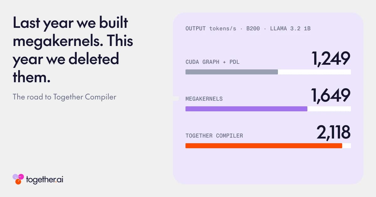
Last year, we helped release some of the first AI megakernels, where we executed an entire model forward pass within a single, highly fused GPU kernel. They reached record breaking speeds, but it was difficult to put them in production. After months of effort, we had a grand total of one model, one batch size, and one customer.
This year, we examined what we could simplify and discovered something surprising. With just CUDA Graphs and PDL on top of default Torch Inductor kernels, we could recover 98% of megakernel performance without writing a single kernel. And with “multi-kernels” and agent loops, we could further beat our old megakernels by up to 1.7x, achieving over 1100 TPS for Llama 1B on H100.
For the past two years, we've been investigating what a next-generation system for inference optimization should look like. After building a series of GPU programming and optimization systems, we arrived at Together Compiler, our framework for continual AI inference optimization. In this blog, we'll revisit the assumptions behind today's compilers, share the experiments that challenged our thinking, and explain the lessons that shaped Together Compiler. Our journey spans three parts:
In Part 1, we show that Torch Compile’s heuristics and benchmarking leave performance on the table, providing motivation to build something radically different.
In Part 2, we revisit the megakernels we built to close that gap, explain why they are not always the right optimization target, and decompose their performance gains into simpler primitives.
In Part 3, we share our “bitter lessons” from crafting agent-driven optimization infrastructure and the final production system we ended up with.
Part 1: Torch Compile
For over a decade, PyTorch has been the foundation of AI development, providing modular, easy-to-use abstractions (nn.Module) that have enabled rapid experimentation. But this modularity comes at a performance cost: executing models as sequences of individual operations can introduce substantial launch overhead, limit opportunities to overlap computation and memory movement, and leave GPU resources underutilized. To address these inefficiencies, PyTorch introduced Torch Compile (“PyTorch 2.0,” powered by Inductor) to optimize and fuse operations, while NVIDIA developed CUDA Graphs to reduce kernel launch overhead. These systems have made enormous progress, but substantial performance gaps remain, often motivating Together’s researchers to invent specialized implementations such as FlashAttention, ThunderKittens, and Megakernels.
We start with a brief overview of how Torch Compile works, then present our findings from investigating Inductor’s internals on Llama 1B.
How Torch Compile Works
At a high level, Torch Compile uses a just-in-time compilation pipeline to capture PyTorch operations into a computation graph, optimize that graph, and generate executable GPU kernels. The key components are:
- Graph capture. TorchDynamo traces Python execution to capture tensor operations in an intermediate representation called an FX graph. During tracing, it uses fake tensors, which carry metadata such as shapes, data types, and strides without allocating or computing the underlying tensor data. This allows the compiler to reason about the computation without actually executing it on the GPU. The resulting FX graph can be transformed and optimized before code generation.
- Operations and kernels. Inductor lowers the captured graph into its own intermediate representation, where operations are organized into categories such as pointwise (e.g., activations), reductions (e.g., summations and softmax), scans (e.g., cumulative sums), and templates (e.g., GEMMs and other specialized compute kernels). Some operations instead invoke existing implementations from libraries such as cuBLAS or custom PyTorch operators. Inductor represents these as external kernels (ExternKernel), whose implementations are generally opaque to its fusion machinery.
- Fusion and optimization. Inductor uses a greedy, pairwise algorithm to decide which operations to fuse into the same kernel. Its can_fuse() function checks whether a candidate fusion is legal, while score_fusion() ranks opportunities using heuristics such as estimated memory traffic savings. The algorithm repeatedly applies profitable fusions, potentially combining many operations into a single kernel. However, these decisions are based on local heuristics rather than a global search over all possible kernel partitions and execution strategies. For example, Inductor may avoid fusing operations that share no memory accesses, even when executing their work together could improve GPU utilization.
On our target Llama 1B workload, Inductor delivers 669 TPS. As we’ll show in Part 2, these generated kernels are sometimes enough, and with small modifications, they can reach similar levels of performance to megakernels. However, on different architectures and newer hardware, Inductor’s heuristics can’t keep up. We investigated where Inductor struggles most and present three findings.
Finding #1: Compiler heuristics cannot reliably select the best implementation across workloads.
Inductor exposes a number of compiler tuning flags that can boost performance. We discovered that even these seemingly simple configurations exposed a surprisingly large and complex search space.
The best optimization depends on the workload. Inductor exposes a freezing flag that tells the compiler that model weights will not change during inference. Knowing this, the compiler can transform the weights ahead of time to make subsequent computations faster. One such transformation converts weights to FP32 to perform certain optimizations, before converting them back to their original, lower-precision format. We found that enabling freezing improved throughput by 10–26% at larger batch sizes, where the GPU performs matrix-matrix multiplications. However, at batch size 1, where inference primarily uses matrix-vector multiplications, enabling the same flag caused a 49% slowdown. Upon inspection, we discovered that the FP32 conversion was not reversed for matrix-vector operations, leaving the GPU to process larger, 32-bit weights instead of the original lower-precision weights. In other words, the exact same compiler optimization could improve performance for one batch size while dramatically degrading it for another.
Optimizations interact in unpredictable ways. As of Q3 2026, Inductor exposes 607 tuning flags, 198 of which were added in the past year. These flags control everything from kernel fusion to memory access patterns and scheduling. Their effects are not independent: enabling the aggressive_fusion flag alone reduced Llama 1B throughput by 6 TPS, but enabling it alongside the combo_kernels, benchmark_fusion, and triton.coalesce_tiling_analysis flags improved throughput by 3 TPS. Even small configuration changes could produce measurable microsecond-level differences in execution time.
Takeaway: the space of possible optimizations and configurations is large, and we should be searching it systematically instead of guessing the right flags to set.
Finding #2: The fastest kernel in isolation isn't necessarily the fastest during inference.
Inductor makes optimization decisions based on its benchmarking harness. We identify two distinct ways that this benchmarking misleads its decision, hurting overall performance as a result.
First, it ignores that kernel performance depends on caching behavior. Torch Inductor clears the GPU's L2 cache before benchmarking individual kernels, but during inference, kernels often reuse data that is cached from preceding operations. We observed 39–58% slower timings in Inductor's isolated benchmarks than in the live forward pass, where cache reuse can reduce memory traffic.
Benchmark inputs can also distort cache behavior in the opposite direction. For example, when benchmarking torch.embedding, Inductor initializes the tensor of token IDs to zero, causing every token to access the same embedding vector. For a 64K-token sequence, this made the kernel 2.1× faster than with random token IDs, due to artificially high cache reuse.
Second, benchmarking overhead can lead to poor kernel selection. Many decode kernels execute in just a few microseconds, making precise timing essential. We found that Inductor's benchmarking harness reported 2.5 µs for an operation that performed no GPU work, while other measurements exceeded the GPU execution times reported by Nsight Systems by approximately 3.6 µs. This is because the harness includes CPU launch overhead after an L2 cache flush, which results in Inductor recording idle time.
These discrepancies lead to faulty compiler decisions. On Llama 1B's output-projection GEMM, Inductor selected a Triton kernel that ran 7.4 µs versus 6.4 µs for cuBLAS in the live forward pass—a 15% slowdown. We also observe this on modern, data-dependent architectures, such as mixture-of-experts architectures like GLM 5.3, where PyTorch’s default benchmarking can be anywhere from 4-21% slower than if we had modified the benchmark to use realistic inputs for the MoE grouped-GEMM kernel (shown in the figure above).
Takeaway: accurate benchmarking requires taking measurements from inside a real forward pass on real input data.
Finding #3: Inductor leaves fusion opportunities on the table.
Inductor’s greedy, pairwise fusion algorithm considers whether two kernels can legally be fused, then evaluates whether fusing them will improve performance. Although repeated pairwise fusion can combine multiple operations, it may miss opportunities that require jointly considering larger groups of kernels or different execution configurations.
We investigated the fusion decisions made by Inductor on Llama 1B and found examples where Inductor keeps kernels separate even when merging them would be beneficial. For example, we found two consecutive kernels (an elementwise activation and a KV indexing kernel) which are simple enough to fuse, but Inductor’s heuristics reject the fusion as they share no memory accesses.
As Inductor evaluates candidates by estimated memory traffic savings, it sees no reason to combine these kernels. However, examining the kernels ourselves, we see that the first kernel launches just six CTAs, meaning that most of the GPU's 132 SMs are idle. Merging these operations into a single launch would help reduce this waste.
Takeaway: an algorithm for kernel fusion should reason about utilization, not just memory.
What these findings pointed to
Each of these findings highlight Inductor limitations that leave the GPU underutilized. Focusing on our broader goal of a next generation system for inference optimization, we turned to the opposite side of the spectrum: megakernels. If we removed compilers entirely, controlling all levels of the stack by hand, where would the performance gains actually come from? By understanding this, we hoped to identify a middle ground, automating megakernel performance with minimal complexity.
Part 2: Megakernels
Since we introduced Megakernels, they have inspired a growing body of work on next-generation AI compilers and GPU execution systems. In this section, we revisit why we built them, how they work, and what happened when we tried to bring them into production.
What motivated megakernels? We observed three sources of inefficiency in conventional inference engines, which typically execute models as sequences of kernels using frameworks such as Torch Compile and CUDA Graphs:
- Kernel launch overhead. Each kernel launch incurs scheduling and dispatch overhead. CUDA Graphs substantially reduce CPU launch overhead, but do not eliminate every cost associated with executing a sequence of separate GPU kernels.
- Limited overlap. Conventional kernel boundaries can prevent useful overlap between operations. For example, the next layer's weights could be prefetched from GPU memory while the current layer is still computing, allowing memory transfers and arithmetic to proceed concurrently.
- Load imbalance. A GPU contains many streaming multiprocessors (SMs), and work is rarely distributed perfectly across them. Some SMs may finish their assigned thread blocks before others, leaving execution resources idle. A more flexible scheduler could redistribute work as SMs become available.
To address these inefficiencies, we designed megakernels around a single persistent GPU kernel that executes an entire model forward pass. Rather than launching a new kernel for each operation, we kept thread blocks resident on the GPU and scheduled successive operations within them. We used specialized warps to coordinate execution, manage resources such as shared memory, and assign units of work to different SMs. We also divided shared memory into fixed-size pages, allowing operations to dynamically allocate and release shared-memory capacity as execution progressed.
The result was a highly optimized execution system capable of eliminating intermediate kernel launches, overlapping work across operations, and dynamically managing GPU resources. On Llama 1B, our megakernel achieved 990 TPS, a 48% improvement over Inductor’s 669 TPS. But it also required building substantial scheduling, synchronization, and memory-management infrastructure ourselves.
Then we tried putting megakernels into production.
At Together AI, during the latter half of 2025, one of our 🐐research team members spent months wrestling with production inference engines: integrating paged KV caches, porting to Blackwell GPUs, debugging race conditions, and handling the many implementation details that arise outside a controlled benchmark.
And after all that effort, we had a grand total of... one Llama 1B megakernel, supporting one batch size (1), one precision (BF16), and one customer.
The performance was impressive. The flexibility was not.
This experience left us with a question: Were megakernels fast because everything ran inside one giant kernel, or because they enabled a handful of valuable optimizations—eliminating launch overhead, overlapping operations, and balancing work across SMs?
To investigate this, we started from Torch Compile at 669 TPS, and systematically ablated each optimization that megakernels provide, one at a time. We found that with only two NVIDIA primitives and default Inductor generated kernels, we could reach equivalent performance with our optimized baseline. This result is surprising, given that many research groups have built far more complex compilers and megakernel systems that fall short of this target. Ultimately, we discovered that megakernels were the wrong objective for a system to target for two main reasons.
First, eliminating kernel launches and overlapping operations doesn’t actually require a megakernel. Second, varying hardwares and modern model architectures expose the megakernel's rigidity and sub-optimality.
Eliminating kernel launch overheads and overlapping operations doesn’t require a megakernel.
Megakernels provide a clean abstraction to enable fine-grained overlap across compute and memory operations. Achieving this overlap comes down to three main things: minimizing kernel launch overhead, reducing tail effects from idle SMs, and overlapping memory prefetching with computation. We examine each of these in detail below, as well as why a singular persistent kernel is not needed to fully achieve these three objectives.
Launch overhead. Kernel launch overhead is costly. In PyTorch, GPU operations pass through ATen dispatch machinery to select a performant implementation based on input shapes, data types, and layouts. This costs 37 microseconds for a H100 Llama 1B down-projection, which is more than double the kernel’s 15 microsecond GPU execution time alone. Stripping PyTorch out entirely and launching pure C++ still costs around 2 microseconds per launch, which adds up across hundreds of kernels in a typical forward pass.
The prescribed solution by PyTorch is CUDA Graphs, a driver-level feature that captures a sequence of GPU operations and replays it with substantially lower CPU launch overhead. In exchange for the captured graph taking up GPU memory, launch overhead reduces to around 1 microsecond. Through this addition, on top of Torch Compile, our Llama 1B performance increases to 864 TPS, 87% of the megakernel.
To further reduce the gap, we explored Programmatic Dependent Launch (PDL), a CUDA mechanism that allows a subsequent kernel to begin executing before its predecessor finishes. Conceptually, PDL allows the hardware to dispatch the next kernel’s thread blocks into SMs as they become free. At the time, Torch Inductor’s Triton backend did not expose the PDL controls we needed, so we compiled the generated kernels down to PTX (NVIDIA's low-level GPU instruction language) and inserted two instructions: griddepcontrol.launch_dependents at the end of each producer kernel, and griddepcontrol.wait at the start of the consumer kernel to ensure synchronization. With these small modifications, our performance reaches 953 TPS, 96% of the megakernel.
For both CUDA graphs and PDL, launch overhead is still nonzero. However, we observe that the megakernel doesn’t get rid of these overheads either; it just trades launch overhead for similar synchronization costs inside the kernel.
In the table above, cost is the time from the end of kernel one to after the end of the synchronization primitive (if applicable) in kernel two. For PDL, counting only time between kernels, the actual kernel gap is 577 ns and 516 ns respectively. Interestingly, intra-kernel synchronization is slightly slower on B200 than H100, as B200 is split into two separate dies. Synchronization cost measured on a single die matches the cost for an equivalent number of SMs on H100.
Compute overlap. Wave quantization occurs when work is not evenly divided across a kernel’s SMs, leaving some SMs idle until the slowest finishes. Megakernels can reduce this waste by allowing a CTA that finishes its operation to begin the next instruction immediately, rather than waiting for the full grid to complete. However, this benefit is limited in practice as layers contain inherent serialization points that no kernel structure can remove.
In our Llama 1B H100 megakernel, three of the five producer-consumer barrier edges per layer require a full barrier, and a fourth is effectively full (a single CTA of the secondary kernel is dependent on 128 CTAs of the previous):
This is significant as it means that the majority of compute warps in a layer often cannot go ahead as they must wait on CTAs from the prior instruction to first complete. These full barriers negate persistent kernels benefits, with a full intra-kernel grid synchronization costing the same as launching an entirely fresh kernel. Modifying our old megaprofiler to capture the start and end of compute warps (not just when an SM first enters), we can see how much useful compute work is accomplished ahead of time. Below shows the idealized overlap that megakernels advertise vs. a more realistic representation. Notably, only the attention instruction is able to take advantage of compute overlap.
Memory overlap. Our earlier megakernel divided each SM’s shared memory into pages that an instruction releases as soon as it finishes with them, enabling the next instruction to begin prefetching its data into the freed space while the current one completes. However, this optimization is worth only 3.3% of the forward’s full execution. Without any memory preloading, our TPS barely drops from 990 to 961.
While the benefit is small, we were curious to see if fancy memory paging mechanisms were necessary to achieve the same degree of memory prefetching wins. To do so, we further pushed PDL through fine-grained placement of its instructions. By inserting the griddepcontrol.wait instruction just before the first read of the predecessor's output, the consumer kernel can preload weights while the previous kernel is still computing. This simple approach enables PDL to recover up to 98% of the gains from paged memory preloading.
Megakernel style preloading also carries additional costs that PDL avoids. Loader warps that are waiting for the previous operation to complete stay resident on the SM and spin. These polls go through the same SM queue that the computing warps use for their warp shuffles, and when this queue fills, the computing warps stall. In the Llama 1B attention-oproj boundary, oproj’s loader warp spins while it waits for the attention operation to finish, adding 1.3 us of overhead compared to naive PDL.
Early weight preloading can also be pointless. Overlapping memory loads only helps when the producer kernel leaves memory bandwidth idle. At the Llama 1B downproj-QKV boundary, bandwidth is already fully saturated, meaning that loading QKV’s weights early slows down downproj by 2.2us but speeds up the QKV operation by a similar amount. Consequently, this pair takes the same time if launched as two separate kernels without any memory overlap.
Our previous Hazy Megakernel enabled lookahead prefetching beyond the immediate next operation. This allowed the Llama 1B up-projection to begin loading in weights while the oproj and attention ops were still completing. PDL alone cannot do this as it assumes a single stream of execution. However, launching dedicated L2 prefetch kernels can achieve a similar effect.
Putting all of this together, default PyTorch Inductor kernels with CUDA graphs and fine-grained PDL are able to achieve 975 TPS, 98% of the hand-written and optimized megakernel baseline, without writing a singular kernel or any complicated intrinsics. With just CUDA graphs and PDL, each of megakernel’s gains from reduced launch overhead and maximized overlap were individually achievable.
Alternative hardwares and modern model architectures expose megakernel's rigidity
Having shown that simple primitives could recover nearly all of the megakernel’s performance, a broader question remained: are megakernels ever not just unnecessary, but suboptimal? We found megakernels monolithic architecture harmful as hardware resource constraints and modern model architectures require flexible, non-static design choices.
Persistent kernels force hardware tradeoffs Megakernels impose a fixed launch envelope across all instructions, restricting kernel design. From warp count to register budget to cluster shape, all operations must match. Registers are allocated per-CTA at schedule time, out of a 65,536-register file per SM. Our H100 Llama-1B megakernel used 20 warps (16 compute warps plus 4 control warps) as short batch-1 decode instructions finish sooner when their rows are spread across more warps. However, heavier tensor-core GEMMs run best with 12 warps. This is as Hopper’s wgmma accumulates into registers, and above 12 warps, the best tiles no longer fit in register memory. If we were to force this operation into the same 20 warp instruction, the GEMMs perform 1.2-1.5x slower. While this isn’t an issue on Blackwell as tcgen05 accumulates in tensor memory, this is still significant as alternative hardwares like AMD run into the same constraints.
Megakernels also add pressure to the SM’s instruction cache, a small buffer that stores machine code that an SM is actively executing. Packing an entire model into a binary is expensive and produces machine code that is often larger than what the instruction cache can hold. To make space when a new operation begins, the SM evicts the previous operation’s instructions. This adds additional overhead, as the kernel must then refetch the evicted instructions from memory when the same operation later repeats.